
Alec Zimmer
Published
July 13, 2021

It's a situation that we've experienced several times: we discover a great feature that substantially improves the quality of one of our fraud models. A model including this feature flags more fraud with substantially higher precision at a threshold we care about, yielding substantial savings in dollars lost. And yet this change may correspond to improvements in AUC or KS that, while statistically significant, appear relatively minor.
Why would these two methods of assessing the value of a fraud score disagree? And, why does a seemingly more technically sophisticated approach to evaluating fraud models generate misleading analysis compared to simply checking the number of dollars lost to high-risk accounts? In this post, we cover a few model metrics commonly used in financial services and discuss some pitfalls of these model metrics in the context of fraud decisioning.
We’ll show that the best way to gauge the value of a new fraud model is to simply check the precision of a score above some threshold and measure the amount of fraud losses.
Background on Modeling Risk
Classical model metrics -- logistic loss, AUC, Gini, KS -- are used across many domains as ways to measure model quality. Aligning on specific metrics as a team is important for comparing the benefit of different features or modeling approaches. Business value, however, is not perfectly correlated with these classical metrics. Let's review the general interpretations of these metrics and later discuss how they align with business value from a fraud detection perspective.
F1 score: the harmonic mean of precision and recall at a cutoff. Intuitively, the harmonic mean is chosen because a model that flags everything at a cutoff (perfect recall, poor precision) and the model that flags nothing at a cutoff (vacuously perfect precision, zero recall) are uninformative models, and should be assigned a value of 0 on this 0 to 1 scale.
AUC: When thinking of modeling the risk of default from a credit product, the interpretation of AUC (“Area Under the ROC Curve”) for a model would be "the probability that a randomly selected account that charges off scores higher than a randomly scored account that repays.”
The Gini index, another commonly reported model statistic, is just the AUC but rescaled to be on a 0-1 scale instead of a 0.5-1 scale, and hence will not be discussed further in this post.
The KS statistic is the maximum difference in cumulative fractions of goods and bads flagged at any possible cutoff.
Logistic loss, also referred to as cross entropy, is generally used as the loss function one is optimizing the model on during training. It is difficult to interpret on an absolute scale, in the way that AUC is known to go from 0.5 to 1. While all metrics are simultaneously a measurement of both the difficulty of the problem and how well the model is doing, the first component especially appears to dominate logistic loss, and the averaged entropy calculations are very difficult to compare across different problems.
With this review in hand, let’s dive into some of the shortcomings of these metrics applied to fraud.
Logistic Loss: Confidence Over-Emphasized
When deciding which model metric a team should focus on optimizing, logistic loss is a natural choice. Its differentiability enables it to be used in training across a wide variety of models, unlike rank-based metrics. Another property that is useful in many domains is that it emphasizes well-calibrated probabilities, unlike a purely rank-based model metric.
But the downside to using logistic loss as an approach to evaluating fraud models is that it penalizes model misses to an extent incommensurate with their business impact. If one is setting a binary threshold and escalating applications that are above the cutoff, then what is most important is whether the fraud cases are above some decisioning threshold. A false negative with probability 0.0001 will be considered twice as bad as a false negative with probability 0.01, although both might be misses at a selected decisioning cutoff. Additionally, no context is provided to the metric for which cutoff is used for decisioning: the difference between 0.09 and 0.11 probabilities for a fraudulent application is quite similar to the difference between 0.11 and 0.13 probabilities, regardless of whether a team is using a cutoff of 0.05, 0.10, or 0.12, each of which has quite different meanings.
Of course the assessed likelihood of fraud does matter to some extent besides whether an application is flagged or not -- higher fraud scores can make it less likely that a fraud attempt slips past some high-risk verification process like manual review, and an extremely low score for a fraudster might suggest that it would be easy for a fraudster to scale up an attack and execute a large volume attack before being caught. Overall though, with fraud systems one generally cares about a 0/1 loss as far as economics go, and logistic loss penalizes extreme losses more heavily than desired.
AUC: Reordering the Bottom 10%
AUC has weaknesses as well when evaluating a fraud model. In general, fraud losses account for a small fraction of losses for financial products, albeit a subset that can be identified with high precision. A fraud model that perfectly predicts 4% of charge-offs and is uncorrelated with other charge-offs would have an AUC around 0.52. Simply introducing some weak variable that is loosely correlated with general credit performance would be able to achieve performance better than this as measured by AUC, but this would not provide marginal benefit to the risk organization. This is true for all fraud models, but AUC makes this distinction especially clear.
To overcome this, fraud teams rightfully focus their development on charge-offs or detected fraud, to avoid the gains in fraud being swamped by spurious changes in credit risk. However, another issue with AUC arises. AUC cares heavily about weighting in the general population, while, as a practical matter, fraud decisioning cares about the precision and recall in the tail of the distribution. Below is an example to make this more concrete.
A good model targets a subset of bad applications with very high precision. Suppose we have a situation where there are 100bps (100 basis points, or 1%) of application fraud, and we have a very weak fraud score that flags 90bps of fraud in the top 5% of applications, and the other 10bps score arbitrarily -- it would have an AUC of roughly 0.92.
Let’s consider two improvements to this model.
- The first causes us to score these 90bps flagged at the very maximum score: the model perfectly predicts fraud for these 90% of the fraudulent apps. The other 10% are unchanged.
- The second improvement causes us to score the bottom 10bps of the fraudulent applications in the 90-95th percentiles. The top 90% of fraudulent applications are unchanged.
Which change offers a larger improvement in AUC?
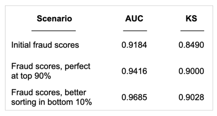
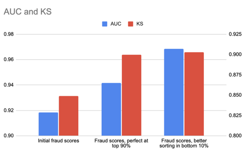
From both an AUC and KS perspective, the second improvement provides the most lift. However, improving the precision of the top 90bps offers much larger business gains -- 90bps of fraud can be perfectly flagged without any false positives, while keeping the remaining population at a rate of approximately 10bps of fraud.
The second improvement which reorders the bottom 10 bps of fraud shows much larger improvements in AUC. It continues to flag 90bps of fraud in the top 5% of applications, and flags the remaining 10bps of fraud with 2% precision, a precision too low to be useful for most purposes. So while the metric improvements are larger, the business gains are likely immaterial.
[Aside: one situation where one would care more about the lower part of the distribution is if this represents an attack vector that can be quickly scaled by a fraud ring, in which case this 10bps of fraud could be scaled up by savvy attackers. Considering these specific situations is outside of the scope of this blog post.]
Since AUC estimates the probability that a randomly selected bad (fraud) scores higher than a randomly selected good (non-fraud), moving a single fraudulent application from the 50th to 55th percentile has roughly the same impact on AUC as moving a single application from the 95th to 99.9th percentile, yet the latter has much greater business relevance.
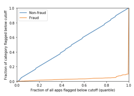
Similarly, this low-score reordering also provides more lift on KS than the other improvement. It gives us a separation of exactly 0.90 in this simulation, albeit, in this case, the difference is much smaller. KS focuses on the greatest distance between curves for the false positives and true positives (plotted below), but, this doesn't generally correspond to a threshold that is economically meaningful - even if it happens to provide a reasonable measure of 0.90 for the specific example in which 90% of the fraud is given the maximum score and the remaining applications are undetected.
An Additional Weakness of KS
The KS statistic is the maximum, across all possible cutoffs, of “the fraction of bad applications (fraud) flagged at this cutoff, minus the fraction of good applications (non-fraud) flagged at this cutoff.” The primary issue with this metric is that this specific threshold may or may not have business relevance.
Suppose that we have some population where we think the threshold examined by the KS statistic is the cutoff we want to use for fraudulent applications, and hence is the threshold of most business relevance. Next, consider the same population but with twice as many fraudulent applications, and assume that the model targets the same rate of fraudulent applications at each score (a very weak assumption). The threshold considered by the KS statistic would stay the same, and the KS value would stay the same. However, we would want to lower the threshold since a lower cutoff would maintain the same marginal break-even point in this scenario with more fraud.
From this example, it's clear the threshold selected by the KS statistic is largely arbitrary.
Our preferred model metric: F1 score
When thinking of the business value provided by a fraud model in terms of loss reduction, the main goal is “maximizing the amount of fraud that would be flagged at a cutoff that maintains a certain marginal precision.” The marginal precision (equivalently, the model’s probability at that cutoff) represents the break-even point at which the lender is indifferent between approving or rejecting (or putting through manual review) this application.
The fraction of total fraud flagged at a cutoff is represented by the recall, and the fraction of applications flagged at that cutoff is the (total, or cumulative) precision. So when the F1 score focuses on maximizing the harmonic mean of precision and recall at a cutoff, it is evaluating how much fraud is captured (normalized by the amount of fraud in the population) and how precisely it is capturing that fraud.
It is possible to weigh precision or recall more heavily with the F_beta score. With our fraud analyses, we have empirically found that the F1 score tends to be maximized at a cutoff that would be economically relevant for many lenders, so choosing the cutoff at which F1 is maximized and looking at this F1 score tends to do quite well in terms of representing the business value provided.
There are practical challenges with F1 score calculation -- it involves estimating the overall amount of fraud in the dataset, which may be nontrivial. But we consider it the best single-number summary of the performance of a fraud model, and estimating the economic losses stopped by a fraud model are even simpler.
The Joy of Fraud Decisioning: Keeping it Simple
Most losses are credit losses, but they’re much more uncertain than fraud losses: there is just more inherent uncertainty whether someone will charge-off or not. With fraud, there can be very large relative improvements to detect fraud with high precision, and this can start to challenge the assumptions built into different model metrics.
In credit underwriting, various model statistics are used to estimate relative performance, but it is challenging to convert these back to the economic or business impact. As we’ve seen, even for a model that is able to make good use of a fraud score, the model improvement measured by a commonly used metric may not correspond to the business impact of the score.
The binary nature of fraud decisioning, however, makes evaluating fraud model performance much more straightforward. The simple method of checking the precision of a score above some cutoff and calculating the amount of fraud losses provides a good estimate of the value provided. In model development, a metric like F1 can help guide improvements, but when assessing business value, the simple approach of selecting a cutoff and estimating the losses is best.
________________________________________

Alec Zimmer leads the data science team at SentiLink, which builds SentiLink’s fraud detection models. Previously he was responsible for verification modeling at Upstart. He has over 400 citations on Google Scholar.
Subscribe
Share
Related Content

Blog article
April 3, 2024
Tips from a Fraud Fighter for Spotting Assumed Identity Abuse
Read article
Blog article
February 29, 2024
Reducing Complexity in Model Risk Management with Attributes
Read article
Blog article
January 18, 2024
What criminals pay to buy stolen identities and tips to keep yours safe
Read article